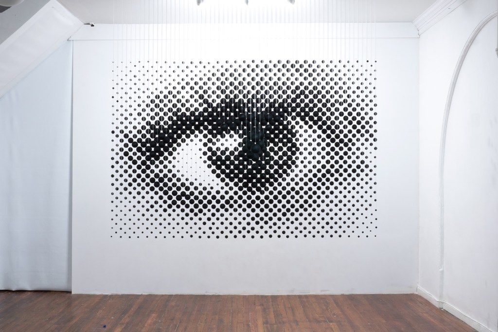
Principal components analysis is all about rotating data. That is all that it does. I know that sounds simple but the algorithm itself is designed to find the best rotation such that most of the variation lies along one axis and the rest of the variation lies along another axis that is perpendicular to the first. These are your principal components that the algorithm is named after.
Here is how I like to think of it. imagine that you have a cloud of data points, like the one below.

Obviously, there is some interesting structure to the data. It almost looks like random noise, but not quite. The data has this tapering thing that it does. Okay, so it is random noise with some heteroscedasticity, sure why not?
Except that what if I told you that under the correct rotation this data turned out to be incredibly organized and not random at all. You might think that I am crazy, however, if we find the correct principal components with which to view this data. You will see just how organized it really is.
It turns out that the “data” we are looking at is a very well known sculpture by artist Michael Murphy. In reality, the cloud of data that we are looking at is a carefully constructed eye.

Under the correct rotations your data is really easy to understand. Here is the moral of the principal component story that we can learn from this sculpture. The data points here are three dimensional, however, if we find the principal components of this data, we can embed our three dimensional structure in two dimensions, and the underlying story that the data is trying to tell us will make far more sense that the full three dimensions ever could.
This is why principal components (and any other decomposition method like independent components, non-negative matrix factorization, factor analysis, and latent dirichlet allocation for that matter) is a powerful feature engineering technique.
If you liked this blog post don’t forget to check out my checklist to see whether or not it makes sense to apply a decomposition method.

Leave a Reply