Last week, I built a multifactor model and ran some optimization to find good candidate zip codes to invest in. This week, I’m looking at the same data again, but this time, we are going to figure out, on a national-level, whether or not our real estate investments are a good hedge against inflation. You may say, well, what we would be shooting for is a positive exposure to inflation. This time, let’s complete our factor model of residential real estate by estimating the 2nd stage regression and recovering factor risk premia.
When we think about inflation, it is usually in a negative connotation. Investors have a relationship with inflation that is largely antagonistic. Inflation will eat into their returns like a mouse nibbling at food stores. Slowly (or sometimes rapidly) diminishing what you thought that you had available to you. Certainly, inflation provides an antagonist with which the investor can struggle. However, in the fight to beat inflation, our enemy gives us an opportunity.
We often think of inflation as a counterbalance to the returns that we are trying to achieve, however, what if inflation contributes to the return that we get? Think about it, if we see inflation in an economy that means that prices are going up. The price of our assets should also go along for that ride as well. Think of it like this, some component of your return is driven by the rate of inflation. Typically, investors think of their returns as uncorrelated with inflation. What my simple little model tells us is that there is a positive correlation between inflation exposures (betas from the first stage) and expected returns.
                            OLS Regression Results
==============================================================================
Dep. Variable:       avg_appreciation   R-squared:                       0.114
Model:                            OLS   Adj. R-squared:                  0.113
Method:                 Least Squares   F-statistic:                     160.3
Date:                Sun, 27 Apr 2025   Prob (F-statistic):          2.88e-129
Time:                        19:58:54   Log-Likelihood:                 11487.
No. Observations:                4998   AIC:                        -2.296e+04
Df Residuals:                    4993   BIC:                        -2.293e+04
Df Model:                           4
Covariance Type:            nonrobust
=================================================================================
                    coef    std err          t      P>|t|      [0.025      0.975]
---------------------------------------------------------------------------------
const             0.0561      0.000    141.940      0.000       0.055       0.057
gdp              -1.1520      0.082    -14.091      0.000      -1.312      -0.992
unemployment     -0.0200      0.015     -1.299      0.194      -0.050       0.010
inflation         0.3025      0.033      9.251      0.000       0.238       0.367
interest_rate     0.4699      0.032     14.804      0.000       0.408       0.532
==============================================================================
Omnibus:                     2269.772   Durbin-Watson:                   2.017
Prob(Omnibus):                  0.000   Jarque-Bera (JB):            20098.299
Skew:                           1.955   Prob(JB):                         0.00
Kurtosis:                      12.012   Cond. No.                         239.
==============================================================================

Notes:
[1] Standard Errors assume that the covariance matrix of the errors is correctly specified.
In fact, the risk premia is 0.3. That’s pretty high. That says that if you bear 1 unit of inflation risk, you are expected to get a return of 30%. That’s not too shabby. That leads me to this distribution for each zip code.

Basically, this distribution shows how residential real estate price appreciation is affected by inflation. Note, that it is actually symmetric about no effect. That’s pretty important. There are some markets where a 1% increase in inflation leads to a 1% increase in real estate prices. There are even a few that run as high as 2%. Some are terrible hedges against inflation (most of them) are not correlated with inflation at all. Then there are the markets that run opposite of inflation. A 1% increase in inflation will lead to a 1% decrease in price appreciation.
So What?
On average, without looking into specific zip codes, residential real estate returns are driven by 3 of our 4 macroeconomic factors. GDP growth, inflation, and interest rates. If you are trying to construct your portfolio in such a way to hedge against inflation, the scourge of investors, residential real estate exposure probably isn’t a horrible way to go. It has a very large inflationary hedge potential. However, you can’t just buy anywhere. As the old adage goes, “location, location, location”. An interesting observation from the regression above, rising GDP seems to moderate the effect of inflation. More income, it appears does not indicate rising prices in real estate. Just an interesting observation.
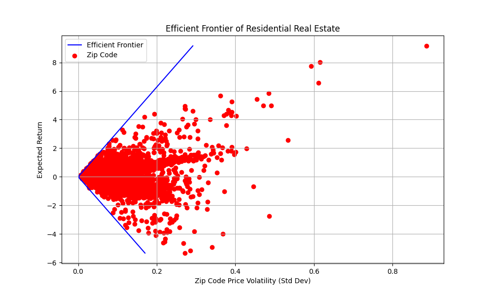
From the model above, we can construct a mean-variance frontier (in this case, it is the mean-standard deviation frontier). We can construct it using the math from the model above. Since we are dealing with a purely linear model, it should come as no surprise that the mean-standard deviation frontier that we calculate is also linear. I then use the data to calculate the expected return for each zip code. Here is what we find:

You may be interested in looking at the code to generate this plot. Note that we use an idiosyncratic error (the error from our time-series stage) as well as systematic errors to construct the efficient frontier so that you can follow along at home. One thing that I would like to point out is that I do not think the linear model does a good job of capturing the frontier for (relatively) larger standard deviations, but we are dealing with simplistic models.
risk_premia = result.params[['gdp', 'unemployment', 'inflation', 'interest_rate']].values
    betas = df[['gdp','unemployment','inflation','interest_rate']]
    # STEP 2: Compute expected returns of assets
    print('Computing expected returns')
    expected_returns = betas @ risk_premia  # (n_assets, )

    # STEP 3: Assume a factor covariance matrix (you could estimate this better)
    # For simplicity, assume factors are uncorrelated with variances of 1
    print('get COV matrix')
    factor_cov = (eco[['gdp','unemployment','inflation','interest_rate']]/100).cov()
    residual_vars = df['resid_var']

    # STEP 4: Compute full asset covariance matrix
    systematic_vars = np.einsum('ij,jk,ik->i', betas, factor_cov, betas)
    total_vars = systematic_vars + residual_vars  # full asset variance
    print(residual_vars)

    # Asset covariance matrix
    cov_matrix = betas @ factor_cov @ betas.T + np.diag(residual_vars)  # (n_assets x n_assets)

    # STEP 5: Set up optimization for frontier
    n_assets = len(expected_returns)
    ones = np.ones(n_assets)

    inv_cov = np.linalg.pinv(cov_matrix.astype('float').fillna(0))  # pseudo-inverse in case it's singular

    # Precompute
    A = ones @ inv_cov @ ones
    B = ones @ inv_cov @ expected_returns
    C = expected_returns @ inv_cov @ expected_returns
    D = A * C - B ** 2

    # Grid of target returns
    target_returns = np.linspace(min(expected_returns), max(expected_returns), 100)

    # Solve for frontier
    frontier_variances = []
    frontier_returns = []

    for r_target in target_returns:
        lam = (C - B * r_target) / D
        gam = (A * r_target - B) / D
        w = lam * (inv_cov @ ones) + gam * (inv_cov @ expected_returns)
        portfolio_return = w @ expected_returns
        portfolio_variance = w.T @ cov_matrix @ w
        frontier_returns.append(portfolio_return)
        frontier_variances.append(portfolio_variance)
    print(systematic_vars)
    # Plot
    plt.figure(figsize=(10, 6))
    plt.plot(np.sqrt(frontier_variances), frontier_returns, label='Efficient Frontier', color='blue')
    plt.scatter(np.sqrt(total_vars), expected_returns, color='red', label='Zip Code')
    plt.xlabel('Zip Code Price Volatility (Std Dev)')
    plt.ylabel('Expected Return')
    plt.title('Efficient Frontier of Residential Real Estate')
    plt.legend()
    plt.grid(True)
    plt.savefig('../../reports/figures/figure1.png')
    plt.close()
The construction of this efficient frontier, gives us an opportunity to evaluate whether or not the real estate holdings that we have contain too much risk. If we aren’t even close to the frontier, we must question whether or not we need to take action to get us closer to the frontier. Now, I get it. You may be saying to yourself, “This is great, but this analysis really feels like overkill. What is the point for the average investor like me?”
To that I say, you can’t buy the whole market. Most real estate investors will buy locally to them. That makes sense from a management perspective, but it can lead to truly terrible investments. An approach like this will help you control risks as you invest in real estate. The goal is to be data driven and to be risk aware when buying investments. This approach helps you develop a portfolio that can move you to an efficient frontier. Furthermore, I did this in this analysis for the national market. It would be fairly trivial to do this for say a geographic area, like a state. This would allow an investor to optimize within a geography if so inclined.
Leave a Reply