Donald’s Terrible Tariff Policy

One of the curses about being an economist, is that everyone asks you about your opinion on economic news. I’ve had so many people ask me about tariffs over the last week. I guess that there is no getting out of this, I need to have an opinion on these proposed tariffs, and what they mean for the rest of us. Here we go: Donald Trump, usurping congressional authority over tariffs is quite concerning. The fact that he thinks that he can unilaterally impose tariffs of this scale is both terrifying and sobering. That means we need to take a look at what the data is telling us about the kind of damage that he can do. So, here we go.

There are lots of reasons why a country may want to impose tariffs on their trading partners. Whether it is to raise government revenue, or to protect an industry it can make a lot of sense at least at first blush to impose a tariff. Back in 2018, I remember telling people that placing a tariff on steel and aluminum actually wasn’t a horrible idea. If the idea was to protect those domestic industries to preserve know-how, and maintain technology from a military perspective, I could get on board. I won’t like it, because it is almost certainly inefficient, but there is some logic beyond the economics. This logic would excuse the terrible economic policy behind the tariff.

However, the recent talk of tariffs is shocking, jarring, and a little idiotic. To say that the tariff policy that Donald Trump unveiled on April 2, 2025 is self-destructive would be an understatement. Now, I am no trade economist, but I have studied enough trade theory to be dismayed. In fact, it was so bad that Trump pressed pause on most of the tariffs because everyone freaked out so hard because of how shockingly bad the policy appeared to be.

Here’s how this post is going to proceed. I am going to introduce a simplistic and highly stylized model of trade. We’ll then estimate the parameters of this model using some data. The hope is that we get to something sensible in terms of parameter values. We can then counterfactually use these estimates to talk about the welfare implications of the announced policies from the Trump administration. What will it mean for consumers? What does it mean for producers, and what will it mean for the government revenues?

Unlike many of the other news and analysis coming out which focused on the equation that the administration published. I will not be focusing on the administration’s use of trade deficit percentage as the choice for how the tariffs were calculated. Instead, I will focus on what the model is telling us about the proposed tariffs.

The Model

As I mentioned above, I will be utilizing a heavily stylized model. For my fellow Econ nerds out there. We will be looking at a partial equilibrium model, with Cobb-Douglas demand functions, and a quadradic producer cost function. The quadradic consumer cost function produces a linear marginal cost function (aka Supply Curve).

Combining Cobb-Douglas Marshallian demand functions with the linear supply curve leads to an equilibrium point which is quadradic in prices. Which means that the solution to the equations can be found analytically. Furthermore, we will use the current duty rates by country to identify the demand curve.

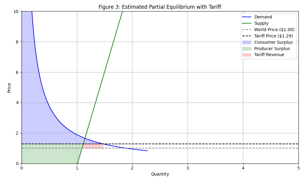
We can then look at the welfare effects of this model. The figure below shows some of the salient features of the model that I just briefly described above. Not marked in the image below are the two deadweight loss “triangles” associated with this model. They would be represented by the white triangles to the left and right of the tariff revenue rectangle.

This model is fairly simplistic, and there are going to be a number of simplifications and exaggerations that I make to estimate the parameters of this model. The goal here is not to build a perfect academic quality journal article. The goal is to build a down and dirty model of trade, that you may have encountered in an entry-level economics course. Granted, people that got economics degrees are more likely to have seen something like this, but it probably isn’t unheard of that somebody completing a general course in economics in college came by a model like this. At the heart of this model is the supply and demand curves and the imposition of a tariff on traded goods. It is not unreasonable that some folks out there came across this model before and you don’t need an advanced graduate degree in economics to fully grasp this model.

Now here are some things that I am going to be assuming in my model, you can pick it apart using any of these assumptions. That’s fine. I don’t care, again, I just want to get a basic understanding here.

First, I am going to assume that all traded goods are homogeneous. Second, I am going to assume that I can aggregate across countries to build a time-series model. This assumption is huge. Technically, for the model that I am looking at, I probably should aggregate trade with the world more carefully and use different types of imports, but hey, we’re not doing this super carefully. We just want to get a flavor for how bad Donald’s proposed tariffs are. We could dig deeper if we really really wanted to, and be more careful, but this is my blog, and it isn’t being peer reviewed, so I’m going to be a bit cavalier about aggregating heterogeneous goods together. However, I will admit that this is the most dangerous assumption that I will make. It is likely the one to cause the model to break down. If you don’t trust this model because of this assumption, you would be wise not to. Third assumption, this model is typically used for a small economy trading with the world. The United States being the largest economy on the planet obviously violates this assumption. I don’t want to hear you whine about that, again, I am trying to use a simplistic model. Fourth and final that I am going to call out, this is a partial equilibrium model, price levels are not chosen endogenously. Do with that what you will. For me this means that the pricing levels are irrelevant. I can utilize the exogeneity to talk solely in terms of relative prices. So I will set the world price equal to $1. This effectively becomes a numeraire for the model allowing it to be tractable and estimable. This restricts me to talking in relative terms to the world price, but due to homogeneity in the supply and demand curves we don’t lose anything so I’m happy to make this assumption.

Last thing before we dive into estimating the model: we need to talk about identification. If you talk to any economist (econometrician really) worth their salt, they will spend a lot of time talking about identification of the model. You need some strategy for doing this because typically we are dealing with equilibrium points. We usually only observe a single quantity and price pair, yet have two equations the supply and demand curve. We can’t write down an equation to map out both curves simultaneously.

Fortunately for us, we have a tariff. This tariff is distorting the market. The distance between the demand and the supply curve (horizontal distance in the graph above) is by definition the quantity imported into the country. So if we subtract the demand from the supply, we can regress this difference on imports and we should be able to map the supply and demand curves simultaneously. Which is really cool. Thus we can identify the demand curve and the supply curve, we will be able to calculate counterfactual consumer surplus, producer surplus, tariff revenue, and deadweight losses for Donald’s proposed tariff regime, and we can decide how much pain Donald is going to cause to American consumers.

Data

So I pulled data from the U.S. Census Bureau on imports and import duties to the United States. This is surprisingly all that we will need to run our models. Important to note is that the traded imports values do not include the tariff duties in the data, so we don’t need to subtract those out. By dividing the tariff duties by the value of the imports, we obtain the current tariff rate. Now if we assume that the world price level is $1 per unit of homogenous good, then we can simply remove the monetary units from the value of the traded goods, and our model will just work.

Note that the rectangle representing tariff revenue is tariff rate multiplied by the quantity imported, which follows from the definition that we utilized to calculate the tariff rate, so everything works out.

Figure 2 shows the value of imports in $10 trillions vs. The tariff rate. Note that there is not a super clear correlation though it does appear to have a negative slope at least unless you discount the last few years which have seen higher import rates due to Trump’s first term tariffs.

Now we made some pretty restrictive assumptions about functional forms for the supply and demand curves. Namely, supply will be linear in price, and demand will be a Cobb-Douglas demand function. Again, the difference between these two values will result in imports. So we set imports equal to the difference between demand and supply, at the price-level (1+t)P_w. P_w is just $1 per unit so the price level is just 1+t or 1 plus the tariff rate.

m = aI/(1+t) - bt - (b+c) + e

Notice something about this equation? If we take the variables to functions of the tariff rate, we have something that is linear in parameters. We can just use ordinary least squares to estimate this equation and we recover all of the parameters of our model. e in the equation above is simply our error term, which we just slapped in to the equation to account for measurement error. We can just as well rewrite this equation as:

m = h_1*(1/(1+t))+h_2*(t)+h_3+e

h_1=aI, h_2=-b, and h_3=-(b+c). Thus, aI=h_1, b=-h_2, and c=h_2 – h_3.

With all of this out of the way, we can get to work estimating a dead simple model that we can utilize to estimate welfare effects of Donald Trump’s proposed tariffs.

Estimation of Model

So like I said, we’ll just use a standard OLS model to estimate this model.

import pandas as pd
import statsmodels.api as sm
import matplotlib.pyplot as plt
import numpy as np

def estimate():
    df = pd.read_csv('../data/Standard Report - Imports.csv', header=2)
    gdp = pd.read_csv('../data/GDP.csv')
    gdp['year'] = pd.to_datetime(gdp['observation_date']).dt.year
    gdp = gdp.groupby('year').max()

    #print(df.columns.values)
    df = df.groupby('Time').sum().reset_index()
    df = pd.merge(df, gdp, how='inner', left_on=['Time'], right_on=['year'])
    print(df.head())
    #df = df[df['Time'] == 2024]
    df['Calculated Duty ($US)']=df['Calculated Duty ($US)']/1e13
    df['Customs Value (Gen) ($US)']=df['Customs Value (Gen) ($US)']/1e13
    df['GDP'] = df['GDP']/10000
    df['Tariff'] = df['Calculated Duty ($US)'].div(df['Customs Value (Gen) ($US)'])
    df['Tariff Discount'] = df['GDP']/(1+df['Tariff'])
    df = df.dropna()
    plt.scatter(df['Tariff'], df['Customs Value (Gen) ($US)'],)
    plt.title('Tariffs vs. Imports')
    plt.xlabel('Tariff Rate')
    plt.ylabel('Value of Imports')
    #df['recession'] = [1 if obj in (2007,2008,2009,2020) else 0 for obj in df['Time']]
    #gf = pd.get_dummies(df,columns=['Time'], drop_first=True)
    model = sm.OLS(endog=df['Customs Value (Gen) ($US)'], exog=sm.add_constant(df[df.columns.values[-2:]]).astype('float'))
    result = model.fit()
    print(result.summary())
    plt.savefig('../output/figures/figure2.png')
    plt.close()
    #print(df['Tariff'].mean())
    return result.params['Tariff Discount'],-result.params['Tariff'],result.params['Tariff']-result.params['const']

if __name__=='__main__':
    print(estimate())

Technically, this works out. Note that I divide everything by $10 trillion dollars. This is just to get the units to a place where I don’t want to hurt myself trying to figure out how to read the output. I get the following output:

                                OLS Regression Results                               
=====================================================================================
Dep. Variable:     Customs Value (Gen) ($US)   R-squared:                       0.941
Model:                                   OLS   Adj. R-squared:                  0.936
Method:                        Least Squares   F-statistic:                     160.6
Date:                       Wed, 16 Apr 2025   Prob (F-statistic):           4.79e-13
Time:                               15:26:43   Log-Likelihood:                 28.504
No. Observations:                         23   AIC:                            -51.01
Df Residuals:                             20   BIC:                            -47.60
Df Model:                                  2                                         
Covariance Type:                   nonrobust                                         
===================================================================================
                      coef    std err          t      P>|t|      [0.025      0.975]
-----------------------------------------------------------------------------------
const               0.1640      0.062      2.642      0.016       0.035       0.294
Tariff            -12.3377      5.474     -2.254      0.036     -23.757      -0.919
Tariff Discount     0.6310      0.046     13.829      0.000       0.536       0.726
==============================================================================
Omnibus:                        1.207   Durbin-Watson:                   1.552
Prob(Omnibus):                  0.547   Jarque-Bera (JB):                0.916
Skew:                          -0.189   Prob(JB):                        0.632
Kurtosis:                       2.098   Cond. No.                         737.
==============================================================================

Notes:
[1] Standard Errors assume that the covariance matrix of the errors is correctly specified.

So do I trust this output? Frankly, no; I do not. This is mainly because I worry that my analysis is overly simplistic, but hey all the signs worked out and I’m pretty happy with the result. It does allow us to analyze the Trump Tariffs and how awful they would really be.

Here is what the model looks like:

I summarize the output of the model in terms of the welfare implications in the table below. For the current tariffs, I use the average tariff from my dataset. For the proposed tariffs, I use 29% average from Donald Trump’s announced tariffs.

	Free Trade	Current Tariffs	Proposed Tariffs
Consumer Surplus	$80.3 Trillion/Year	$80.0 Trillion/Year	$75.5 Trillion/Year
Producer Surplus	$73.9 Trillion/Year	$74.0 Trillion/Year	$77.1 Trillion/Year
Government Revenue	None	$100 Billion/Year	$1 Trillion/Year
Deadweight Loss	None	$100 Billion/Year	$600 Billion/Year
Total Surplus	$154.2 Trillion/Year	$154.2 Trillion/Year	$153.6 Trillion/Year

In other words, we will be harming consumers to the tune of $4.5 Trillion per year. Most of that will be transferred to producers. Domestic producers will receive an additional $3.1 Trillion in profits under the proposed tariffs. The government will get about $1 Trillion in additional revenue. Somewhat surprisingly to me, the economy will only lose about $600 billion in losses due to these tariffs.

So these tariffs will bring in about 10X the revenue for the government, but consumers are going to pay the price for sure. We can compare the burden of the tariffs as percentage as well. In other words, what percent of the tariff burden will be born by producers, and what percentage would be born by consumers?

It turns out according to this model, 92.64% of the burden of these tariffs will be born by consumers. Ouch!

Incidentally, a 65% tariff would push the country to autarky. So this gets us about half-way to complete self-sufficiency where the United States would basically be forced to produce everything for itself rather than import goods.

Normative Final Thoughts

I’m surprised by how efficient the tariffs look like they will be. The total surplus under free trade is $154.2 Trillion and the deadweight loss looks like it would only be around $600 Billion. This represents a loss in efficiency of roughly 0.39%. That’s not too bad all things considered. We could probably afford to do that, so I’m not terribly opposed on the efficiency grounds. The tariffs aren’t going to hurt too badly.

The tariffs are highly regressive. 92.64% of the burden of these new tariffs will be born by consumers. On this basis alone it is obvious that this is a transfer from working class people to the richest and most elite people in the country. We will be taking $4.5 Trillion from the American public and transfer it to domestic businesses. Essentially, these tariffs will create artificial monopolies for domestic producers, and we will transfer the lion’s share of that money to the rich elite through higher prices. It is immoral and outrageous that we would do this to our own people. I am outraged by this proposed tariffs and the harm that they would do to the American people. It is irresponsible and shows the reckless disdain that Donald Trump has for you and I.

I do not see any strategic value in these tariffs. They appear to be nothing more than blatant protectionist malarkey that is full of jingoism and nationalist rhetoric. I think that this is a major problem for our country. I am glad that we pressed pause for 90 days (good), but geez, we need to step away from this suicidal policy beyond the 90 day pause.

Incidentally, the POTUS should not even have the ability to unilaterally impose tariffs, ever! I find it highly unconstitutional. Congress should get off their butts and strip the POTUS of any authority to impose tariffs. The framers of the constitution specifically gave that power to the legislative branch, and that is where it belongs. Nobody should unilaterally be capable of causing the turmoil that Trump caused this last week.

For the nerds that want to calculate welfare effects, ya’ll can figure out the math and the economics, here’s the rest of the code that I used:

import numpy as np
import matplotlib.pyplot as plt
from estimation import estimate
from scipy.optimize import root_scalar

def run(tau, params):
    p_world = 1       # World price (lower than autarky)
    alpha = params[0]
    I = 3
    a = params[1]
    b = params[2]
    # Derived prices
    p_tariff = p_world * (1 + tau)

    # Marshallian demand: q = αI / p
    def demand(p):
        return alpha * I / p

    # Profit-maximizing supply: MC = P ⇒ dC/dq = 2cq = p ⇒ q = p / (2c)
    def supply(p):
        return (p-b)/a


    def excess_demand(p):
        return demand(p) - supply(p)

    star = root_scalar(excess_demand, bracket=[1, 100], method='bisect')
    print(f"P_star: {star.root}")
    pstar = star.root
    Qstar = demand(pstar)
    print(f"Q_star: {Qstar}")


    # Equilibrium quantities
    q_d_free = demand(p_world)
    q_s_free = supply(p_world)
    imports_free = q_d_free - q_s_free

    #producer_burden = (q_s_free-q_star)*p_world -

    q_d_tariff = demand(p_tariff)
    q_s_tariff = supply(p_tariff)
    imports_tariff = q_d_tariff - q_s_tariff

    consumer_burden = alpha * I * np.log(q_d_free) - alpha * I * np.log(q_d_tariff) - (q_d_free - q_d_tariff) * p_world + (p_tariff-p_world)*(q_d_tariff-Qstar)

    producer_burden = 0.5*(p_tariff-p_world)*(q_s_tariff-q_s_free)+(p_tariff-p_world)*(Qstar-q_s_tariff)

    cburden = 100*consumer_burden/(consumer_burden+producer_burden)
    pburden = 100*producer_burden / (consumer_burden + producer_burden)
    # Welfare calculations
    def consumer_surplus(p, q):
        return alpha * I * np.log(q)-alpha*I*np.log(0.01) - p * q

    def producer_surplus(p, q):
        return p * q - a/2 * q**2 -b*q

    cs_free = consumer_surplus(p_world, q_d_free)
    ps_free = producer_surplus(p_world, q_s_free)

    cs_tariff = consumer_surplus(p_tariff, q_d_tariff)
    ps_tariff = producer_surplus(p_tariff, q_s_tariff)
    gov_rev = p_world * tau * imports_tariff

    ts_free = cs_free + ps_free
    ts_tariff = cs_tariff + ps_tariff + gov_rev
    dwl = ts_free - ts_tariff

    # Plotting
    q_vals = np.linspace(0.01, q_d_free * 1.2, 500)
    p_demand_vals = alpha * I / q_vals
    p_supply_vals = a * q_vals+b

    plt.figure(figsize=(10, 6))
    plt.plot(q_vals, p_demand_vals, label="Demand", color="blue")
    plt.plot(q_vals, p_supply_vals, label="Supply", color="green")
    plt.axhline(p_world, color='gray', linestyle='--', label=f"World Price (${p_world:.2f})")
    plt.axhline(p_tariff, color='black', linestyle='--', label=f"Tariff Price (${p_tariff:.2f})")

    # Welfare shading under tariff
    plt.fill_between(q_vals[q_vals <= q_d_tariff],
                     alpha * I / q_vals[q_vals <= q_d_tariff],
                     p_tariff, color='blue', alpha=0.2, label='Consumer Surplus')
    plt.fill_between(q_vals[q_vals <= q_s_tariff],
                     p_tariff, a * q_vals[q_vals <= q_s_tariff]+b,
                     color='green', alpha=0.2, label='Producer Surplus')
    plt.fill_between([q_s_tariff, q_d_tariff],
                    p_world, p_tariff,
                    color='red', alpha=0.2, label='Tariff Revenue')
    # plt.fill_between([q_s_tariff, q_d_tariff],
    #                  p_tariff, p_demand_vals[(q_vals > q_s_tariff) & (q_vals < q_d_tariff)],
    #                  color='gray', alpha=0.2, label='Deadweight Loss')

    # Annotations
    #plt.axvline(q_s_tariff, color='green', linestyle=':', label="Domestic Supply (Tariff)")
    #plt.axvline(q_d_tariff, color='blue', linestyle=':', label="Domestic Demand (Tariff)")
    #plt.axvline(q_d_free, color='blue', linestyle='--', alpha=0.4)
    #plt.axvline(q_s_free, color='green', linestyle='--', alpha=0.4)

    plt.title("Figure 3: Estimated Partial Equilibrium with Tariff")
    plt.xlabel("Quantity")
    plt.ylabel("Price")
    plt.legend(loc="upper right")
    plt.grid(True)
    plt.tight_layout()
    plt.xlim(0,2)
    plt.ylim(0,4)
    plt.savefig('../output/figures/figure3.png')

    # Print welfare results
    print(f"--- Welfare Analysis ---")
    print(f"Consumer Surplus (Free Trade):     {cs_free:.2f}")
    print(f"Producer Surplus (Free Trade):     {ps_free:.2f}")
    print(f"Total Surplus (Free Trade):        {ts_free:.2f}")
    print()
    print(f"Consumer Surplus (With Tariff):    {cs_tariff:.2f}")
    print(f"Producer Surplus (With Tariff):    {ps_tariff:.2f}")
    print(f"Government Revenue:                {gov_rev:.2f}")
    print(f"Total Surplus (With Tariff):       {ts_tariff:.2f}")
    print(f"Deadweight Loss:                   {dwl:.2f}")
    print()
    print(f"Consumer Burden Share:                   {cburden:.2f}%")
    print(f"Producer Burden Share:                   {pburden:.2f}%")

if __name__=='__main__':
    run(.0147, estimate())
    run(0.29, estimate())