Logistic regression was like magic the first time that I saw it. I grasped the utility almost immediately, but then I was shown how to hang economic theory on top of logistic regression and my face melted! Then I learned about the assumptions in logistic regression that no one seems to talk about like the assumption of the independence of irrelevant alternatives. I’m actually a little shocked that nobody talks about this super important assumption for this model in the data science blogs.
That’s why I’ve been wanting to write this post for a while but I am just getting around to it. It’s been on the back burner since I was working on my book, and while I was putting together this free guide to data science in six easy steps. (You can get it by clicking that link or just enter your email in the form below). So I haven’t gotten around to writing up this tutorial until now.
At any rate, I am really excited to talk about logistic regression. In fact, while I was doing my PhD, I spent most of my time working with these types of models. Ultimately, I didn’t use them in my dissertation, but I learned so much about these models it is scary. At any rate, let’s take a look at how to perform logistic regression in R.
The Data
I’m going to use the hello world data set for classification in this blog post, R.A. Fisher’s Iris data set. It is an interesting dataset because two of the classes are linearly separable, but the other class is not. So it gives you the opportunity to try to find interesting classifiers. It is also why it has stood the test of time, and it gets used so often.
library(nnet)
data <- iris
attach(data)
The code above loads everything that we need into the instance of R. And this dataset is relatively clean, so I think that we can go ahead and throw down a quick model. Before we do, let's just take a quick peek at the data:
head(data)
Which gives you this output:
  Sepal.Length Sepal.Width Petal.Length Petal.Width Species
1          5.1         3.5          1.4         0.2  setosa
2          4.9         3.0          1.4         0.2  setosa
3          4.7         3.2          1.3         0.2  setosa
4          4.6         3.1          1.5         0.2  setosa
5          5.0         3.6          1.4         0.2  setosa
6          5.4         3.9          1.7         0.4  setosa
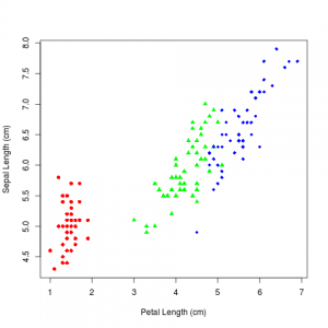
And then you can visualize the data with this command:
plot(Sepal.Length ~ Petal.Length,
       xlab = "Petal Length (cm)",
       ylab = "Sepal Length (cm)",
       pch = c(16, 17, 18)[as.numeric(Species)],  # different 'pch' types
       main = "Iris Dataset",
       col = c("red", "green","blue")[as.numeric(Species)],
       data = iris)
Which produces this image:
The Classic Binary Logistic Regression
Now I'm going to do something that is quite silly. I'm going to start by ignoring one of the classes from the analysis so that I am modeling just a simple binary outcome. The reason that I am going to go ahead and do this is quite simple, I want to illustrate the IIA (independence of irrelevant alternatives) property of logistic regression. The IIA property is one of those things that nobody talks about, but it really is one of the most important assumptions about logistic regression.
So let me describe the problem in a little more detail. Imagine that you have a model that decides whether or not to ride the blue bus or take the car. It works perfectly, and tells you what you would be the happiest to do on any given day. Now imagine that a red bus gets introduced by the city. The classifier now needs to decide between blue bus, red bus, or car. Well to satisfy the IIA property, I have to essentially draw my choices for red bus "equally" from the distribution of choices that I would have made in the absence of red bus. In other words, if 50% of the time I would have chosen blue bus and 50% of the time I would have taken my own car under the original scenario, when I get to the new model, I will choose car 33% of the time, blue bus 33% of the time, and red bus 33% of the time. This is clearly wrong. I should choose car 50% of the time, and blue bus 25% of the time, and red bus the other 25% of the time.
So let's start by making just one class, specifically we'll take Setosa as the positive class. We'll do this by creating a dummy variable, called "Setosa".
Setosa <- as.numeric(Species == "setosa")
At this point we have everything that we need to run a binary logistic regression. We can do so with this code:
model <- glm(Setosa ~ Sepal.Length + Petal.Length, family=binomial(link=logit))
summary(model)
This code will produce the following results:
Deviance Residuals:
       Min          1Q      Median          3Q         Max
-4.063e-05  -2.100e-08  -2.100e-08   2.100e-08   4.767e-05

Coefficients:
              Estimate Std. Error z value Pr(>|z|)
(Intercept)     -78.26  316177.72   0.000    1.000
Sepal.Length     39.83   81738.89   0.000    1.000
Petal.Length    -48.60   43659.68  -0.001    0.999

(Dispersion parameter for binomial family taken to be 1)

    Null deviance: 1.9095e+02  on 149  degrees of freedom
Residual deviance: 5.0543e-09  on 147  degrees of freedom
AIC: 6

Number of Fisher Scoring iterations: 25
What's going on under the hood? We are fitting a generalized linear model, specifically we are using a binomial maximum likelihood with a logistic transformation. That is what you see with family=binomial (telling it to use a binomial likelihood function) and link=logit (telling it to use a logistic transformation). Also don't worry about the warnings that come with this, it is because it is a linearly separable class from the other two.
But Wait What About The Third Class?
Technically speaking we are taking the difference of the positive and negative class when we do logistic regression. I won't go into the nitty-gritty details here. But I will point you towards an excellent resource if you want to dig into the guts of logistic regression. It is Kenneth Train's book on discrete choice models: Discrete Choice Methods With Simulation. This book is phenomenal and frankly if you use logistic regression it is worth at least a read, and Train has posted the entirety of the book for free on his website, Thank You Dr. Train!
At any rate, now we'll choose a base class, and take differences with respect for that for the other classes. We'll do this using the command "multinom" from the nnet package. Notice that it is a multinomial likelihood as opposed to a binomial likelihood, that's where multinomial logistic regression gets its name.
Species <- relevel(Species, ref='virginica')
model2 <- multinom(Species ~ Sepal.Length + Petal.Length)
summary(model2)
Which gives you this output:
Call:
multinom(formula = Species ~ Sepal.Length + Petal.Length)

Coefficients:
           (Intercept) Sepal.Length Petal.Length
setosa        11.09551    17.871555    -29.85965
versicolor    39.72135     4.003423    -13.27159

Std. Errors:
           (Intercept) Sepal.Length Petal.Length
setosa       334.42913    93.637848    63.225678
versicolor    13.03843     1.618022     3.894181

Residual Deviance: 23.85705
AIC: 35.85705
So what is going on here? I should have gotten the same coefficients or at least something close to it for setosa class. While this is where that pesky IIA property comes into play. It is drawing examples from versicolor from both setosa and virginica classes, in a 1:2 proportion, thanks to IIA. If you look at the scatter plot you will notice it is kind of like we introduced a red bus/blue bus situation by breaking versicolor and virginica apart. Which has messed up the coefficients. So you have to be aware of this property of logistic regression.
Now what to do about it? Well, all of these are out of the scope for this blog post. There are a couple of things that you can try. I would personally suggest a probit model where you specify the correlation matrix between the classes. This does involve a bit of hubris, because you basically have to say that you know what the correlation between the classes should be. Or you can try your hand at building a nested logistic regression (this is basically building a constrained neural network from my point of view, you can argue with me about this point in the comment section if you like). Or you can build a mixed logit model, which is a powerful and extremely flexible version of logistic regression where you allow parameters at an instance level to vary. You do this by assuming that each instance draws from a parameter distribution. For some problems that can be very theoretically appealing, especially when you have heterogeneous agents or some other gobbledy-gook. I may revisit some of these models later. But for now just realize that this is how you deal with IIA issues.
The full code
library(nnet)
data <- iris
attach(data)

head(data)

plot(Sepal.Length ~ Petal.Length,
       xlab = "Petal Length (cm)",
       ylab = "Sepal Length (cm)",
       pch = c(16, 17, 18)[as.numeric(Species)],  # different 'pch' types
       main = "Iris Dataset",
       col = c("red", "green","blue")[as.numeric(Species)],
       data = iris)

Setosa <- as.numeric(Species == "setosa")
model <- glm(Setosa ~ Sepal.Length + Petal.Length, family=binomial(link=logit))
summary(model)

Species <- relevel(Species, ref='virginica')
model2 <- multinom(Species ~ Sepal.Length + Petal.Length)
summary(model2)
